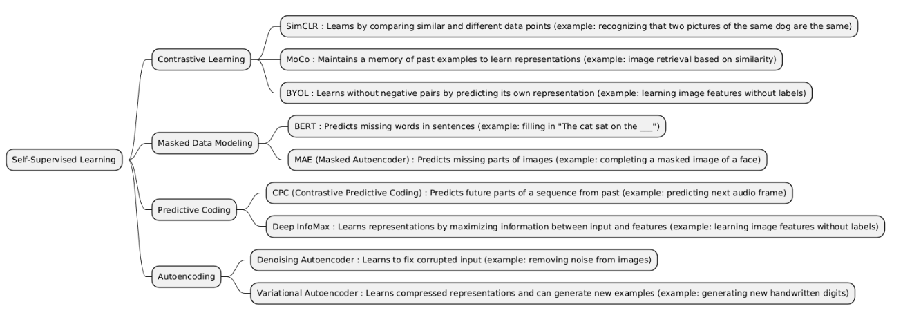
Self-Supervised Learning is a type of machine learning where the system generates its own labels from the input data. By creating pretext tasks, the model learns useful representations from unlabeled data, which can then be applied to downstream tasks like classification or prediction.
| Type | What it is | When it is used | When it is preferred over other types | When it is not recommended | Examples of projects that is better use it incide him |
|---|---|---|---|---|---|
| Contrastive Learning | Contrastive Learning is a type of Self-Supervised Learning that learns useful data representations by comparing pairs of samples. The idea is to make the representations of similar samples close together in the learned space, and different samples far apart. | It is used when you have a lot of unlabeled data and want to learn rich representations that can later be used for tasks like classification, retrieval, or segmentation. It’s widely used with images, text, and audio. |
• Better than Masked Data Modeling when masking parts of the data isn’t practical (like full images or audio clips). • Better than Predictive Coding when you want general representations not tied to sequential order. • Better than Autoencoding because it focuses on discriminative representations instead of just reconstructing inputs. |
• When you have very little data. • When it’s hard to define what counts as “similar” or “different.” • When the main goal is prediction or generation, not representation learning. |
• Training a model like SimCLR or MoCo to learn image embeddings without labels, then using them for classification. • A music recommendation system using contrastive learning to learn song similarity. |
| Masked Data Modeling | Masked Data Modeling is a technique where parts of the input (words, pixels, etc.) are hidden (masked), and the model learns to predict the missing parts. It helps the model understand the structure and context of data. | Used when data has strong internal structure (like text or images). Common in NLP (e.g., BERT) and vision (e.g., Masked Autoencoders). |
• Better than Contrastive Learning when you don’t want to define “positive/negative” pairs. • Better than Predictive Coding for non-sequential data (e.g., images). • Better than Autoencoding because it forces deeper contextual understanding instead of simple reconstruction. |
• When data lacks clear internal context (e.g., tabular data). • When masking too much breaks meaning or structure. • When you have very small datasets — models can overfit. |
• BERT: predicting masked words in sentences. • Masked Autoencoders (MAE): predicting masked image patches to learn visual features. |
| Predictive Coding | Predictive Coding is an approach where the model learns to predict future or missing parts of data sequences based on past context. It’s often used to capture temporal or sequential dependencies in data. | Used when data is sequential or time-dependent (videos, audio, sensor data, text). The goal is to learn representations that understand temporal structure. |
• Better than Masked Data Modeling for time-based data (e.g., predicting next frames or sounds). • Better than Contrastive Learning when sequential prediction gives richer context. • Better than Autoencoding when you care about future prediction, not reconstruction. |
• Not good for non-sequential or static data (like single images). • When future prediction isn’t meaningful (e.g., random unordered datasets). • When latency matters — prediction models can be computationally heavy. |
• CPC (Contrastive Predictive Coding): predicting future audio segments from past ones. • Video frame prediction: predicting next frames in a video for representation learning. |
| Autoencoding | Autoencoding is a method where a model learns to compress input data into a lower-dimensional latent representation (encoding) and then reconstruct it back (decoding). | Used when you want to learn efficient data representations, reduce noise, or perform dimensionality reduction without labels. |
• Better than Contrastive Learning when you need direct reconstruction of inputs. • Better than Masked Data Modeling for continuous data (e.g., images, audio). • Better than Predictive Coding for non-sequential or static data. |
• Not ideal when representations need to be discriminative (e.g., for classification). • Reconstruction loss can make it focus on low-level details, not semantics. • Not suitable for time-dependent tasks or long-range dependencies. |
• Image Denoising Autoencoder — clean noisy images by learning reconstruction. • Anomaly Detection in credit card transactions — train autoencoder to reconstruct normal data, anomalies reconstruct poorly. |
import numpy as np
from sklearn.semi_supervised import LabelPropagation
from sklearn.metrics import accuracy_score
from transformers import AutoTokenizer, AutoModel
import torch

# 1️⃣ Example text data
texts = [
    "I love machine learning",
    "Python is great for AI",
    "I hate bugs in code",
    "Debugging is frustrating",
    "AI is the future",
    "I dislike slow computers"
]

# Labels: 1 = positive, 0 = negative, -1 = unlabeled
labels = np.array([1, 1, 0, 0, -1, -1])

# 2️⃣ Load pre-trained BERT model
tokenizer = AutoTokenizer.from_pretrained("distilbert-base-uncased")
model = AutoModel.from_pretrained("distilbert-base-uncased")

# 3️⃣ Encode text into embeddings
def get_embedding(text):
    inputs = tokenizer(text, return_tensors="pt", truncation=True, padding=True)
    with torch.no_grad():
        outputs = model(**inputs)
    return outputs.last_hidden_state.mean(dim=1).squeeze().numpy()

X = np.array([get_embedding(t) for t in texts])

# 4️⃣ Apply Label Propagation
label_prop_model = LabelPropagation()
label_prop_model.fit(X, labels)

# 5️⃣ Predicted labels
predicted_labels = label_prop_model.transduction_
print("Predicted labels:", predicted_labels)

# 6️⃣ If you know true labels for evaluation
true_labels = np.array([1, 1, 0, 0, 1, 0])
accuracy = accuracy_score(true_labels, predicted_labels)
print("Accuracy:", accuracy)
import torch
import torch.nn as nn
import torchvision
import torchvision.transforms as transforms
from sklearn.semi_supervised import LabelPropagation
from sklearn.metrics import accuracy_score
import numpy as np

# 1️⃣ Simple image dataset (CIFAR-10 subset)
transform = transforms.Compose([
    transforms.Resize((32, 32)),
    transforms.ToTensor()
])

dataset = torchvision.datasets.CIFAR10(root='./data', train=True, download=True, transform=transform)
loader = torch.utils.data.DataLoader(dataset, batch_size=64, shuffle=True)

# 2️⃣ Simple SimCLR-like encoder
class SimpleSimCLR(nn.Module):
    def __init__(self, feature_dim=128):
        super().__init__()
        self.encoder = nn.Sequential(
            nn.Flatten(),
            nn.Linear(32*32*3, 512),
            nn.ReLU(),
            nn.Linear(512, feature_dim)
        )
    def forward(self, x):
        return self.encoder(x)

model = SimpleSimCLR()
model.eval()

# 3️⃣ Extract embeddings
N = 20
X = []
y = []
for i, (img, label) in enumerate(loader):
    if i*N >= N: break
    embeddings = model(img).detach().numpy()
    X.append(embeddings)
    y.append(label.numpy())
X = np.vstack(X)
y = np.hstack(y)

# 4️⃣ Make some labels unknown (-1)
y_semi = y.copy()
y_semi[10:] = -1

# 5️⃣ Apply Label Propagation
label_prop_model = LabelPropagation()
label_prop_model.fit(X, y_semi)
predicted_labels = label_prop_model.transduction_

# 6️⃣ Evaluate
accuracy = accuracy_score(y, predicted_labels)
print("Predicted labels:", predicted_labels)
print("Accuracy:", accuracy)
import torch
import torch.nn as nn
import torch.nn.functional as F
from sklearn.semi_supervised import LabelPropagation
from sklearn.metrics import accuracy_score
from torchvision import datasets, transforms
from torch.utils.data import DataLoader
import numpy as np

# 1️⃣ Define a simple VAE
class VAE(nn.Module):
    def __init__(self, input_dim=784, hidden_dim=256, latent_dim=2):
        super().__init__()
        self.fc1 = nn.Linear(input_dim, hidden_dim)
        self.fc_mu = nn.Linear(hidden_dim, latent_dim)
        self.fc_logvar = nn.Linear(hidden_dim, latent_dim)
        self.fc2 = nn.Linear(latent_dim, hidden_dim)
        self.fc3 = nn.Linear(hidden_dim, input_dim)

    def encode(self, x):
        h = F.relu(self.fc1(x))
        return self.fc_mu(h), self.fc_logvar(h)

    def reparameterize(self, mu, logvar):
        std = torch.exp(0.5*logvar)
        eps = torch.randn_like(std)
        return mu + eps * std

    def decode(self, z):
        h = F.relu(self.fc2(z))
        return torch.sigmoid(self.fc3(h))

    def forward(self, x):
        mu, logvar = self.encode(x)
        z = self.reparameterize(mu, logvar)
        return self.decode(z), mu, logvar

# 2️⃣ Load MNIST
transform = transforms.Compose([transforms.ToTensor(), transforms.Lambda(lambda x: x.view(-1))])
mnist = datasets.MNIST(root='./data', train=True, download=True, transform=transform)
loader = DataLoader(mnist, batch_size=128, shuffle=True)

# 3️⃣ Initialize VAE
vae = VAE()
vae.eval()

# 4️⃣ Get embeddings for first N samples
X_list = []
y_list = []
N = 100
for i, (imgs, labels) in enumerate(loader):
    with torch.no_grad():
        mu, _ = vae.encode(imgs)
        X_list.append(mu.numpy())
        y_list.append(labels.numpy())
    if len(X_list)*128 >= N:
        break

X = np.vstack(X_list)[:N]
y = np.hstack(y_list)[:N]

# 5️⃣ Make some labels unknown (-1)
y_semi = y.copy()
y_semi[50:] = -1

# 6️⃣ Apply Label Propagation
label_prop = LabelPropagation()
label_prop.fit(X, y_semi)
predicted_labels = label_prop.transduction_

# 7️⃣ Evaluate
accuracy = accuracy_score(y, predicted_labels)
print("Predicted labels:", predicted_labels)
print("Accuracy:", accuracy)